
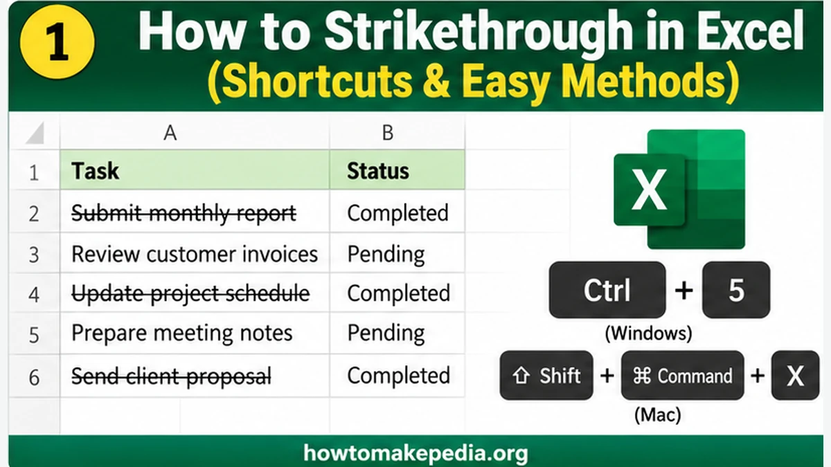

To strikethrough in Excel, select a cell and press Ctrl + 5 on Windows or Shift + Command + X on Mac. This adds a line through the text without deleting it. Press the same shortcut again to remove the line.
You can also use the Format Cells menu, cross out part of a cell, or automatically strike through completed tasks. Here’s how each method works.
Quick Answer: Excel Strikethrough Shortcuts
| Platform | Shortcut or Method | Result |
|---|---|---|
| Windows | Ctrl + 5 | Adds or removes strikethrough |
| Mac | Shift + Command + X | Adds or removes strikethrough |
| Excel for the web | Home > Font Settings > Strikethrough | Applies or removes strikethrough |
| Windows Format Cells | Ctrl + 1 | Opens formatting options |
| Mac Format Cells | Command + 1 | Opens formatting options |
These shortcuts are listed in Microsoft’s Excel keyboard shortcut documentation.
What Is Strikethrough in Excel?
Strikethrough is a font effect that places a horizontal line through text or numbers while leaving the original content in place.
For example, a task tracker might contain:
| Task | Status |
|---|---|
| Completed | |
| Review customer invoices | Pending |
| Completed |
The crossed-out tasks remain readable, making it easy to see what’s finished without losing previous information.
Strikethrough is useful for completed tasks, canceled appointments, outdated prices, reviewed records, and finished projects.
Important: Strikethrough doesn’t delete data or change its underlying value. A crossed-out number can still be included in Excel formulas.
Method 1: Use the Strikethrough Keyboard Shortcut
The keyboard shortcut is the quickest method when you need to cross out one or several cells.
How to Strikethrough in Excel on Windows
- Open your Excel workbook.
- Click the cell containing the text you want to cross out.
- Press Ctrl + 5.
- The selected cell’s contents will appear with a line through them.
- Press Ctrl + 5 again to remove the effect.
For example, if cell A2 contains “Prepare presentation,” selecting A2 and pressing Ctrl + 5 marks the task as completed without changing its text.
How to Strikethrough in Excel on Mac
On a Mac, use a different shortcut:
- Open Excel and select the cell.
- Press Shift + Command + X.
- Check whether the text is crossed out.
- Repeat the shortcut to toggle the effect off.
If the shortcut doesn’t respond, check for keyboard conflicts or use Format Cells instead.
How to Strikethrough Multiple Cells

You don’t need to format completed tasks individually.
- Select the cells you want to format, such as A2.
- Press Ctrl + 5 on Windows or Shift + Command + X on Mac.
- Excel applies strikethrough to the selected cells.
You can also select a rectangular range such as A2 if you want to cross out task names, owners, and statuses together.
The shortcut affects the selected cells, not necessarily the entire worksheet row.
Method 2: Apply Strikethrough Using Format Cells

If you prefer using menus, the Format Cells dialog provides a straightforward alternative.
Step-by-Step Instructions
- Select the cell or range you want to format.
- Press Ctrl + 1 on Windows or Command + 1 on Mac. You can also right-click the selection and choose Format Cells.
- Open the Font tab.
- Find the Effects section.
- Check the Strikethrough box.
- Click OK.
Excel applies the effect immediately.
This method is useful when you also want to change font color, font size, or other formatting settings.
You can also open the Font dialog using the small dialog launcher in the Home tab’s Font group.
Method 3: Strikethrough Only Part of a Cell
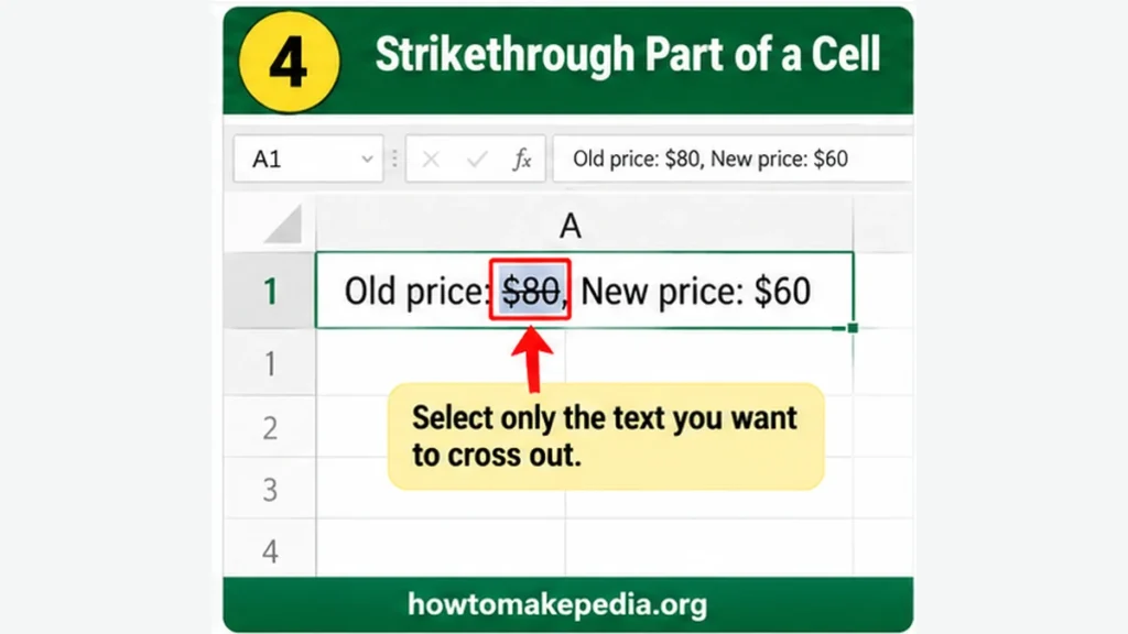
Sometimes you want to cross out one phrase while keeping the rest of the cell unchanged.
Suppose cell B2 contains:
Old price: $80, New price: $60
You want only “$80” crossed out, like this:
Old price: $80, New price: $60
How to Format Selected Characters
- Double-click cell B2 to enter editing mode.
- Highlight only “$80” within the cell.
- Open the Font settings using the Home tab’s Font dialog launcher.
- Under Effects, select Strikethrough.
- Click OK, then finish editing the cell.
Only the highlighted characters should have strikethrough formatting.
You can use the same approach to mark an outdated word in a note or an old deadline in a text entry.
Limitation: Character-level formatting is best suited to text entered directly into a cell. Excel doesn’t support formatting individual characters in a numeric value or formula result in the same way. Browser-based editing features may also differ from desktop Excel.
Method 4: How to Strikethrough in Excel Online
You can apply strikethrough directly in Excel for the web without downloading your spreadsheet or opening the desktop application.
According to Microsoft’s Excel for the web instructions, follow these steps:
- Open your workbook in Excel for the web.
- Select the cells containing the text.
- Click the Home tab.
- In the Font group, select Font Settings.
- In the formatting dialog, select Strikethrough.
- Click OK.
To remove the effect, return to the same settings and deselect Strikethrough.
The browser interface may vary depending on your Excel version and ribbon layout. Don’t assume every desktop shortcut will behave the same way in a browser.
Method 5: Automatically Strikethrough Completed Tasks With Conditional Formatting
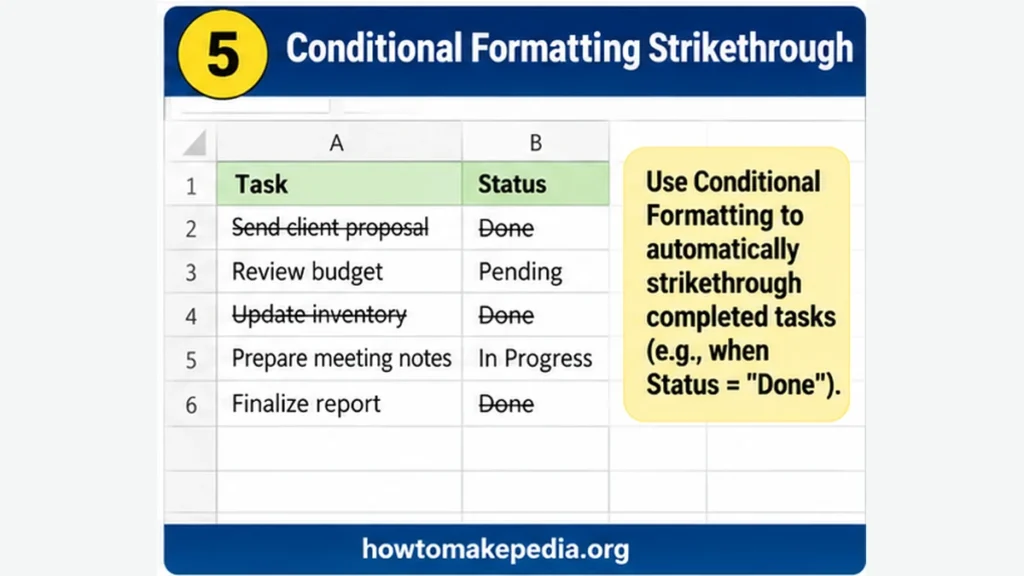
If you maintain a task tracker, applying strikethrough manually every time something is finished can become tedious.
Conditional Formatting lets Excel apply it automatically when a status changes.
Step 1: Create a Task Tracker
Set up a worksheet with these columns:
| Row | A: Task | B: Owner | C: Status |
|---|---|---|---|
| 2 | Send client proposal | Emma | Done |
| 3 | Review budget | Olivia | Pending |
| 4 | Update inventory | James | Done |
| 5 | Prepare meeting notes | Sophia | In Progress |
Step 2: Select the Entire Target Range
Select A2.
This range covers your task descriptions, owners, and statuses for up to 99 task rows.
If you want only the task names crossed out, select A2 instead.
Step 3: Create a Conditional Formatting Rule
- Go to Home > Conditional Formatting > New Rule.
- Select Use a formula to determine which cells to format.
- Enter this formula:
=$C2="Done"
- Click Format.
- Open the Font tab.
- Check Strikethrough.
- Click OK to confirm the formatting.
- Click OK again to save the rule.
Step 4: Understand the Formula
The formula checks whether the Status cell in column C contains “Done.”
$Ckeeps the Status column fixed.2identifies the first data row.- The row reference adjusts automatically as Excel evaluates each subsequent row.
"Done"is the condition that triggers the formatting.
The rule must start at row 2 because your selected range begins at A2.
Step 5: Check the Result
When you change C3 from “Pending” to “Done,” Excel automatically crosses out the cells in A3.
If you change the status back to “Pending,” the conditional strikethrough disappears, provided no other formatting is applying it.
To confirm the range, open Home > Conditional Formatting > Manage Rules and check that Applies to is:
=$A$2:$C$100
This makes the rule practical for task trackers, project checklists, and approval logs.
How to Strikethrough an Entire Row in Excel
There are two practical methods.
Manual method: Select the data cells across the row, such as A5, and use your platform’s strikethrough shortcut.
Automatic method: Use the conditional formatting formula =$C2="Done" with the target range A2, as explained above.
The automatic method is especially helpful when several people update the same task tracker.
Avoid selecting entire worksheet rows unnecessarily. If your table only contains three columns, formatting those columns is usually enough.
If you frequently cross out text, adding a command to the Quick Access Toolbar can be more convenient than remembering a shortcut.
In supported Windows desktop versions:
- Open Excel and choose File > Options.
- Select Quick Access Toolbar.
- Change the command list to Commands Not in the Ribbon or All Commands.
- Find Strikethrough.
- Select it and click Add.
- Click OK.
You can now use the command from the toolbar when it is available in your version.
You can also customize the Ribbon by creating a new group and adding the Strikethrough command. Excel for Mac has separate Ribbon and toolbar customization settings, so the exact steps may differ.
How to Remove Strikethrough in Excel
Removing strikethrough depends on how it was originally applied.
Remove Manual Strikethrough
Select the affected cells and press:
- Windows: Ctrl + 5
- Mac: Shift + Command + X
You can also open Format Cells > Font and uncheck Strikethrough.
Remove Automatic Strikethrough
If a conditional formatting rule is responsible:
- Select the affected range.
- Open Home > Conditional Formatting > Manage Rules.
- Locate the rule applying strikethrough.
- Edit or delete the rule.
- Confirm your changes.
Alternatively, use Conditional Formatting > Clear Rules > Clear Rules from Selected Cells.
Be careful with Home > Clear > Clear Formats. This removes other formatting as well, including colors, borders, and number formats.
Strikethrough vs. Diagonal Borders in Excel
Strikethrough and diagonal borders serve different purposes.
Strikethrough adds a horizontal line through the characters in a cell. It’s suitable for marking a task as completed or identifying an old value.
A diagonal border draws a diagonal line across the cell area. It doesn’t follow the shape or length of the text.
For example, strikethrough works well for a canceled order description. A diagonal border might be useful to mark a cell as not applicable in a printed form.
To add a diagonal border, open Format Cells > Border and select a diagonal border option.
These two formatting features aren’t interchangeable.
Why Is Strikethrough Not Working in Excel?
Several common issues can prevent strikethrough from appearing or being removed.
1. The Shortcut Does Nothing
Make sure you’re using the shortcut for your operating system.
Try Format Cells > Font > Strikethrough if the keyboard shortcut doesn’t work. Also check whether another application or keyboard setting is intercepting the keys.
2. You’re Editing a Cell
Selecting a complete cell and selecting characters inside it are different actions.
Press Enter or Escape to leave editing mode before applying strikethrough to an entire cell. For partial text formatting, highlight the characters while editing.
3. The Wrong Range Is Selected
Check the selected cell addresses. If only A2 is selected, formatting won’t automatically extend to B2 and C2.
Select the complete range you want to cross out.
4. Conditional Formatting Keeps Reapplying It
A formatting rule may be responsible for the effect.
Open Conditional Formatting > Manage Rules and check the rule conditions and the Applies to range. Edit or remove the rule if necessary.
5. The Browser Handles the Shortcut
When working in Excel for the web, use the available Font Settings instead of relying on desktop keyboard shortcuts.
6. A Formula Result Has an Unexpected Strikethrough
In some Microsoft 365 versions, Excel may automatically cross out a formula result because it is a stale value that hasn’t been recalculated.
This can occur in Manual or Partial Calculation modes.
Try recalculating with F9 or Formulas > Calculate Now. Don’t assume the line was added as ordinary font formatting.
7. Only Part of the Text Needs Formatting
Double-click the cell, select the specific characters, and apply the Font effect instead of formatting the entire cell.
Does Strikethrough Affect Excel Formulas?
No. Ordinary strikethrough formatting changes appearance, not the stored number or how a formula calculates it.
Suppose your worksheet contains:
| Cell | Value |
|---|---|
| A2 | 100 |
| A3 | |
| A4 | 300 |
Enter:
=SUM(A2:A4)
Excel still returns 600, even though A3 appears crossed out.
If you want to exclude canceled entries from totals, use a separate Status column.
For example, with amounts in A2 and statuses in B2, you could use:
=SUMIF(B2:B4,"Active",A2:A4)
This adds only the amounts whose status is “Active.”
Strikethrough alone doesn’t tell Excel which numbers to ignore.
Excel Strikethrough Methods Compared
| Method | Best For | Automatic? | Limitation |
|---|---|---|---|
| Keyboard shortcut | Fast manual formatting | No | Platform-specific |
| Format Cells | Menu-based formatting | No | Requires several clicks |
| Partial-cell formatting | Old prices or text corrections | No | Best for manually entered text |
| Excel for the web | Browser-based spreadsheets | No | Interface may vary |
| Conditional Formatting | Completed task trackers | Yes | Requires a correctly configured rule |
| Custom toolbar button | Frequent manual formatting | No | Customization varies by version |
Common Mistakes to Avoid
Most strikethrough problems come from a few avoidable mistakes.
- Expecting data to disappear: Strikethrough doesn’t delete anything.
- Expecting calculations to ignore crossed-out values: Use formulas and a status column instead.
- Using Windows shortcuts on Mac: Follow the platform-specific shortcut.
- Formatting the wrong range: Check the selection before applying the effect.
- Confusing borders with strikethrough: A diagonal border crosses the cell area, not just its contents.
- Clearing all formatting: Remove only the effect you don’t want.
- Ignoring existing rules: Conditional formatting can keep bringing the line back.
- Using the wrong formula reference: Match your formula’s first row to the selected range’s first row.
Frequently Asked Questions
What is the shortcut for strikethrough in Excel?
Press Ctrl + 5 on Windows or Shift + Command + X on Mac after selecting the cell.
How do I strikethrough in Excel on Mac?
Select the cell and press Shift + Command + X. Alternatively, open Format Cells with Command + 1 and select Strikethrough under Font effects.
How do I cross out text without deleting it?
Apply strikethrough formatting. The original text remains in the cell.
Can I strikethrough in Excel Online?
Yes. Select the cells, go to Home > Font Settings, and enable Strikethrough.
How do I strikethrough only part of a cell?
Double-click the cell, highlight the intended characters, and apply strikethrough through Font settings in a supported desktop version.
How do I strikethrough multiple cells?
Select the complete range, then use the strikethrough shortcut or Format Cells.
How do I automatically strikethrough completed tasks?
Use Conditional Formatting with a formula such as =$C2="Done" applied to your task table.
How do I strikethrough an entire row?
Select the cells across the row and apply strikethrough. For automatic formatting, use a rule based on the row’s Status cell.
Why is Ctrl + 5 not working?
Check that you’re using Excel for Windows, select the intended cells, and make sure another program or keyboard setting isn’t handling the shortcut.
How do I remove strikethrough formatting?
Repeat the relevant shortcut or deselect Strikethrough in Format Cells. For automatic formatting, edit or delete the conditional rule.
Does strikethrough affect Excel formulas?
No. Crossed-out numbers remain part of normal calculations unless your formulas explicitly exclude them.
Yes, supported desktop versions allow toolbar or Ribbon customization. The available commands and settings can vary.
Conclusion
The fastest way to strikethrough in Excel is Ctrl + 5 on Windows or Shift + Command + X on Mac. If you prefer menus, use Format Cells > Font > Strikethrough.
For a frequently updated task list, Conditional Formatting is a better choice because the line can appear or disappear automatically when the task status changes. Use the method that fits how you manage your worksheet.

2 Comments
Pingback: How to Wrap Text in Excel: Easy Steps & Shortcuts
Pingback: How to Insert Bullets in Excel: 6 Easy Methods