


To make a histogram in Excel, select your numerical data, click the Insert tab, choose Insert Statistic Chart, and select Histogram. Excel automatically groups your numbers into intervals, helping you see how often values occur.
You can also adjust the histogram’s bin width, change the number of bins, or create a frequency distribution using Analysis ToolPak or the FREQUENCY function.
Quick Answer: How to Create a Histogram in Excel
Follow these five steps:
- Enter your numerical data into an Excel column.
- Select the cells containing the numbers.
- Click the Insert tab.
- Select Insert Statistic Chart > Histogram.
- Right-click the horizontal axis and choose Format Axis to customize the bins.
Your histogram is ready. You can now adjust its appearance and examine how your values are distributed.
What Is a Histogram in Excel?
A histogram is a chart that shows how numerical values are distributed across different ranges, called bins.
For example, imagine you have test scores for 20 students. Instead of examining every score separately, you could create a histogram showing how many students scored between 50 and 59, 60 and 69, and so on.
A histogram contains two main axes:
- Horizontal axis: Displays the numerical intervals.
- Vertical axis: Shows how many observations fall within each interval.
Each bar represents a group of values. Taller bars indicate that more observations fall within that range.
Histograms are useful for analyzing test scores, customer ages, delivery times, product measurements, and other numerical data.
Before Creating a Histogram: Prepare Your Data
A histogram works best when your worksheet contains accurate numerical observations.
Let’s use a sample of 20 student test scores.
Enter Test Score in cell A1, then place the following numbers in A2:A21:
72, 55, 85, 61, 95, 77, 67, 83, 52, 74, 98, 64, 81, 58, 79, 91, 70, 88, 75, 69
Before creating the chart, review your worksheet:
- Put one numerical observation in each cell.
- Keep the measurements in one column.
- Check for numbers accidentally stored as text.
- Remove unintended totals or summary rows.
- Confirm that your selected range contains every required observation.
Check for accidental duplicates: Repeated values are not necessarily errors. Two students may legitimately receive the same score, and both should be counted.
However, imported datasets sometimes contain accidentally duplicated records. If that happens, follow our guide on how to remove duplicates in Excel after verifying which records should actually be deleted.
Also, avoid mixing individual measurements with group averages. A histogram of 20 student scores answers a different question from a histogram of 20 class averages.
Method 1: Make a Histogram With Excel’s Built-In Chart
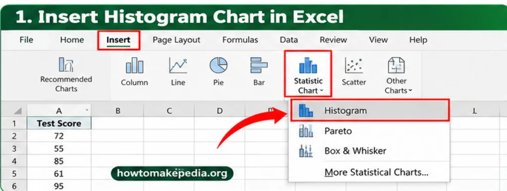
Excel’s built-in Histogram chart is the fastest option for beginners because it automatically groups numerical observations.
Step 1: Select the Numerical Data
Open your Excel worksheet and select cells A2 containing the 20 test scores.
Make sure you select the numerical values rather than an unrelated column.
Step 2: Open the Insert Tab
Click the Insert tab on the Excel ribbon.
This tab contains the tools for creating charts, tables, illustrations, and other worksheet elements.
Step 3: Choose the Histogram Chart
Find Insert Statistic Chart in the Charts group.
Select:
Insert > Insert Statistic Chart > Histogram
Excel creates a histogram using the selected numerical data.
You can also find Histogram through the available chart types in the Insert Chart dialog.
Step 4: Understand the Chart
Look at the two axes.
The horizontal axis displays the score intervals, while the vertical axis indicates how many scores fall within each interval.
Excel determines the bin width automatically unless you specify another setting.
Step 5: Customize the Histogram
Right-click the horizontal axis and select Format Axis.
Under Axis Options, you can change the bin width, specify the number of bins, or configure overflow and underflow categories.
Step 6: Verify the Distribution
Check that your chart uses the intended 20 scores and does not include any summary totals or unrelated cells.
Remember that Excel’s automatically generated intervals may differ from the manually defined ranges used later in this guide.
How to Change Histogram Bin Width in Excel

Bin width determines how much of the numerical scale each histogram interval covers.
For example, a width of 10 represents score intervals spanning 10 points.
To change the bin width:
- Click the histogram.
- Right-click its horizontal axis.
- Select Format Axis.
- Open Axis Options.
- Choose Bin Width.
- Enter a positive number, such as 10.
Excel updates the chart to reflect your selection.
What Happens With a Smaller Bin Width?
Smaller bins usually create more bars. They can reveal smaller variations, but may also make the histogram look crowded.
What Happens With a Larger Bin Width?
Larger bins usually produce fewer bars. They can make broad patterns easier to see, but may hide meaningful differences.
Important: Setting the bin width to 10 does not guarantee that Excel will use exactly the ranges 50–59, 60–69, and 70–79. Interval alignment also matters.
How to Change the Number of Bins in Excel
Instead of choosing the width of each interval, you can tell Excel how many bins you want.
- Right-click the horizontal axis.
- Select Format Axis.
- Open Axis Options.
- Select Number of Bins.
- Enter the number you want.
- Review the updated chart.
Excel adjusts the intervals according to the selected number.
For a small dataset, try a few reasonable settings and compare the results. There is no universal number of bins that works best for every histogram.
How to Use Underflow and Overflow Bins
Underflow and overflow bins help group observations outside selected boundaries.
Underflow Bin
An underflow bin combines values less than or equal to a specified number.
For example, setting an underflow boundary of 60 groups all scores of 60 or below together.
Overflow Bin
An overflow bin combines values greater than a specified number.
For example, an overflow boundary of 90 groups scores above 90 into one category.
To enable either setting, open Format Axis > Axis Options, select the appropriate checkbox, and enter the boundary.
These options can be helpful when highlighting unusually low or high values. However, grouping extreme values together can also hide differences between them.
Method 2: Create a Histogram Using Analysis ToolPak
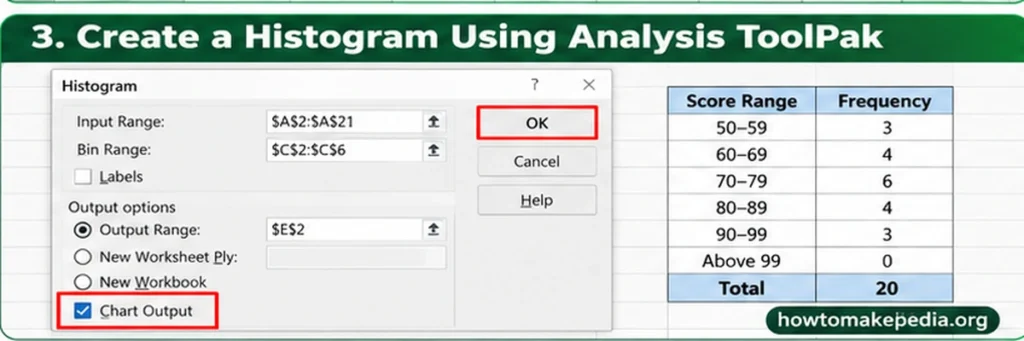
Analysis ToolPak is useful when you want a frequency table with specific numerical bin boundaries.
Unlike automatic histogram binning, this method lets you supply the exact upper limits for the intervals.
Step 1: Enable Analysis ToolPak
In supported Excel versions for Windows:
- Go to File > Options > Add-ins.
- Select Excel Add-ins from the Manage menu.
- Click Go.
- Check Analysis ToolPak.
- Click OK.
The Data Analysis command should appear on the Data tab.
Step 2: Prepare Your Data and Bins
Keep the 20 student scores in A2.
Enter these upper bin limits into C2:C6:
59, 69, 79, 89, 99
Each number represents the highest value included in that bin.
Step 3: Open the Histogram Tool
Go to:
Data > Data Analysis > Histogram
Click OK.
Step 4: Configure the Histogram
Enter these settings:
- Input Range: $A$2:$A$21
- Bin Range: $C$2:$C$6
- Output: Choose a new worksheet or suitable empty output range.
- Chart Output: Check this option to generate a chart.
Leave Labels unchecked because the input ranges contain numbers only.
Click OK.
Step 5: Check the Frequency Results
Your frequency distribution should look like this:
| Score Range | Frequency |
|---|---|
| 50–59 | 3 |
| 60–69 | 4 |
| 70–79 | 6 |
| 80–89 | 4 |
| 90–99 | 3 |
| Above 99 | 0 |
| Total | 20 |
The first bin includes values up to 59. Each later bin includes values greater than the previous boundary and less than or equal to its own upper limit.
Step 6: Verify Your Total
The frequency counts should add up to 20.
For example, if your five main frequency counts appear in cells E2, enter:
=SUM(E2:E6)
The result should be 20.
If you’re unfamiliar with this formula, our guide on how to sum in Excel explains how to total cells, rows, and columns.
Step 7: Review the Chart
If you selected Chart Output, Excel also generates a chart based on the calculated frequencies.
The Analysis ToolPak produces a generated result rather than a live FREQUENCY formula. If your original scores change, you may need to run the analysis again.
Method 3: Make a Histogram Using the FREQUENCY Function
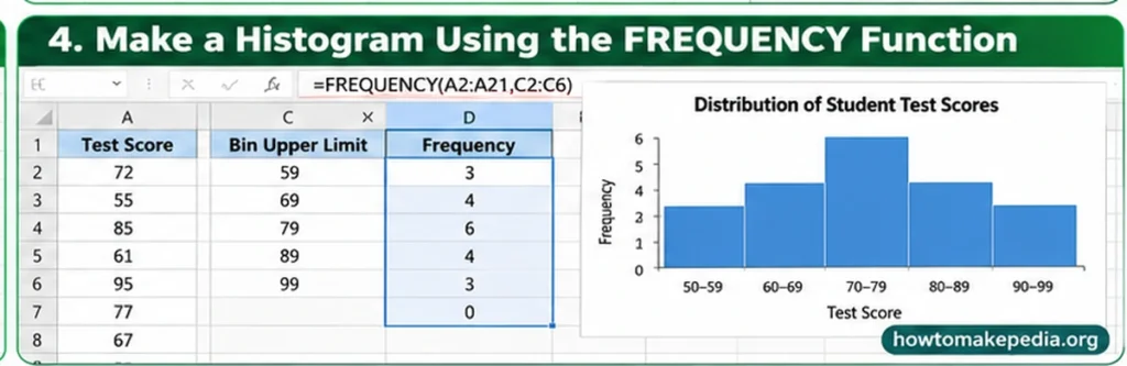
The FREQUENCY function counts how many numerical observations fall within specified upper bin boundaries.
This method is useful when you need formula-based frequency counts.
Step 1: Enter the Original Data
Keep the sample scores in cells A2.
Step 2: Define the Bin Boundaries
Enter the following numbers in C2:C6:
59, 69, 79, 89, 99
Step 3: Enter the FREQUENCY Formula
Click cell D2 and enter:
=FREQUENCY(A2:A21,C2:C6)
In current Excel versions supporting dynamic arrays, press Enter.
The results should spill into D2:D7:
3, 4, 6, 4, 3, 0
The final result counts values above 99.
In older Excel versions without dynamic-array spilling, select D2, type the formula, and confirm it using Ctrl + Shift + Enter.
Step 4: Create a Chart From the Frequency Table
Enter the interval labels into E2 and reference the corresponding counts in F2.
Then:
- Select E2.
- Click Insert.
- Choose a 2-D Column Chart.
- Add an appropriate chart title.
- Set the series Gap Width to 0 if you want adjoining bars for equal-width, contiguous intervals.
This creates a column chart from your frequency table rather than Excel’s built-in statistical Histogram chart.
When the original data changes, the FREQUENCY formula recalculates under normal automatic calculation settings.
How to Choose the Right Histogram Bin Size
The best bin size depends on your data.
Consider the number of observations, the numerical range, measurement units, and the detail you want to show.
For the 20 student scores, intervals of 10 points provide a useful summary.
Using very narrow intervals might produce many nearly empty bars. Using only two wide intervals could hide differences between students’ scores.
Try several bin widths and choose the one that explains the distribution without hiding meaningful information.
For fair comparisons between two datasets, use consistent bin boundaries whenever possible.
How to Customize a Histogram in Excel
A few changes can make your histogram easier to understand.
Change the Chart Title
Select the chart title and enter something descriptive, such as:
Distribution of Student Test Scores
Add Axis Titles
Select the chart and use Chart Design > Add Chart Element > Axis Titles, where available.
Use:
- Horizontal axis: Test Score
- Vertical axis: Frequency
Adjust the Chart Appearance
Choose readable colors, resize the chart as needed, and check that the interval labels are easy to read.
Avoid unnecessary 3-D effects or heavy decorative styling. These can make the distribution harder to interpret.
How to Read a Histogram
Start by finding the tallest bar. It represents the interval containing the most observations.
In our manually defined frequency table, the 70–79 interval contains six scores, making it the most populated group.
You can also examine whether the observations are concentrated near the center, spread widely, or clustered toward one end.
Unusually isolated bars may indicate extreme observations worth reviewing.
A histogram reveals patterns in numerical data, but it does not explain what caused those patterns.
Histogram vs. Bar Chart: What’s the Difference?
Although histograms and bar charts look similar, they serve different purposes.
| Feature | Histogram | Bar Chart |
|---|---|---|
| Data | Numerical measurements | Usually categories |
| Horizontal axis | Numeric intervals | Category labels |
| Bars | Show frequencies in intervals | Compare category values |
| Order | Numeric sequence | Can often be rearranged |
| Gaps | Usually adjoining for equal-width bins | Usually separated |
| Example | Distribution of test scores | Sales by product |
A frequency-table-based column chart can represent histogram data when constructed appropriately.
However, simply removing the gaps between bars does not automatically turn an ordinary categorical chart into a statistically meaningful histogram.
How to Make a Histogram in Excel on Mac
Excel for Mac also supports Histogram charts in supported versions.
- Select your numerical data.
- Open Insert.
- Click the statistical chart icon.
- Choose Histogram.
- Customize the chart using the available formatting controls.
To enable Analysis ToolPak on a supported Mac version, open Tools > Excel Add-ins, select Analysis ToolPak, and click OK. Restart Excel if prompted.
Menu labels and layout may differ slightly between Excel versions.
How to Make a Histogram in Excel Online
In supported versions of Excel for the web, select your numeric data and look for Insert > Statistical > Histogram.
Depending on the web interface and workbook compatibility, some chart creation or formatting controls may differ from desktop Excel.
If the required option is unavailable, you can create a frequency table using supported formulas and display it with a column chart. Another option is to open the workbook in desktop Excel to create or edit the Histogram chart.
Why Is My Excel Histogram Not Working?
Several common problems can affect histogram results.
1. Histogram Option Is Missing
Check your Excel version and available chart types. Older versions may not have the built-in Histogram command.
2. Numbers Are Stored as Text
Imported scores can look numerical but behave as text. Convert them to actual numbers before charting.
3. Wrong Data Range
Check that the selected range contains only the intended observations.
4. Bin Width Looks Incorrect
Open Format Axis > Axis Options and review the selected bin settings.
5. Too Many or Too Few Bars
Try a different bin width or number of bins.
6. Blank Cells Are Present
Check whether missing observations are intentional. Blank cells and text can cause the counted observations to differ from your expected total.
7. Analysis ToolPak Is Missing
Enable it through Excel’s Add-ins settings in a supported desktop version.
8. FREQUENCY Returns an Extra Number
This is normal. The additional result counts observations above the highest specified bin boundary.
9. FREQUENCY Shows #SPILL!
Clear any cells blocking the formula’s output range. Dynamic arrays need sufficient empty space.
10. The Chart Doesn’t Update
Built-in charts generally respond to source-data changes, while generated Analysis ToolPak output may need to be recreated. FREQUENCY formulas normally recalculate when the source cells change.
11. The Frequency Counts Look Wrong
Check the upper bin boundaries, source range, and numbers stored as text. Remember that each upper limit is inclusive.
12. Bars Have Large Gaps
If you created a regular column chart from a frequency table, review the series Gap Width setting.
Common Mistakes When Making a Histogram
Avoid these problems when preparing your chart:
- Choosing categories instead of numerical observations.
- Including a total row in the source range.
- Removing legitimate repeated measurements.
- Selecting bins that hide useful differences.
- Ignoring unexpected extreme values.
- Comparing charts with inconsistent interval boundaries.
- Treating group averages as though they were individual observations.
- Assuming Analysis ToolPak output updates automatically.
Checking the original data and your interval settings will prevent many of these errors.
Frequently Asked Questions
How do I make a histogram in Excel?
Select your numerical data and choose Insert > Insert Statistic Chart > Histogram in supported desktop versions.
What data do I need for a histogram?
You need numerical observations, such as test scores, ages, measurements, or delivery times.
Where is the Histogram chart option?
Look under the Insert tab in the statistical chart options. The menu varies by Excel version.
How do I change histogram bin width?
Right-click the horizontal axis, select Format Axis, and change Bin Width under Axis Options.
How do I change the number of bins?
Open Format Axis, select Number of Bins, and enter your preferred number.
What are underflow and overflow bins?
They group observations at or below a lower boundary, or above an upper boundary.
Can I use Analysis ToolPak to create a histogram?
Yes. On supported desktop versions, enable Analysis ToolPak and choose Data > Data Analysis > Histogram.
What does the FREQUENCY function do?
FREQUENCY counts observations within numerical ranges defined by upper bin limits.
Why does FREQUENCY return one extra result?
The final result counts values above the highest specified bin boundary.
Can I create a histogram from a frequency table?
Yes. You can display interval labels and counts in a column chart, with appropriate formatting.
Can I make a histogram in Excel on Mac?
Yes. Supported Excel for Mac versions provide a Histogram chart option.
Can I create a histogram in Excel Online?
Supported Excel web interfaces offer statistical chart options, although some controls can differ from desktop Excel.
Why are my histogram frequencies incorrect?
Check your input cells, numerical formatting, bin limits, and selected ranges.
How do I add labels to an Excel histogram?
Select the chart and use Chart Design or the available chart element controls to add chart and axis titles.
Does a histogram update automatically?
A built-in histogram is linked to its source values. Analysis ToolPak results generally require rerunning the tool after the data changes.
How many bins should a histogram have?
There is no fixed answer. Choose intervals according to dataset size, range, and how clearly they display the distribution.
Conclusion
Making a histogram in Excel is straightforward once your numerical data is organized correctly. The built-in Histogram chart is the fastest method for most beginners.
Use Analysis ToolPak when you want a frequency report with specified boundaries, or the FREQUENCY function when you need formula-based counts.
Whichever method you choose, review your bin settings and confirm that the chart accurately represents your observations. A clear histogram can make patterns in a long list of numbers much easier to understand.
