


To sum numbers in Excel, click an empty cell, type =SUM(A2:A10), and press Enter. Excel will add the values from A2 through A10. For an even faster method, select the cell below your numbers and click AutoSum on the Home tab.
You can use these methods for sales reports, monthly budgets, expenses, and everyday calculations. This guide explains how to total rows, columns, separate cells, and filtered data, along with ways to fix common SUM formula problems.
What Does SUM Mean in Excel?
SUM is a built-in Excel function that adds numbers together. Instead of typing a long calculation with plus signs, you can tell Excel which cells to include.
The basic syntax is:
=SUM(number1,[number2],...)
Here is what each part means:
- SUM: The function that performs addition.
- number1: The first number, cell reference, or range.
- number2: Optional additional numbers or ranges.
- Colon (:): Identifies a continuous range of cells.
- Comma (,): Separates individual references or ranges.
For example, =SUM(B2:B6) adds five cells in column B.
If your business records daily sales in those cells, Excel calculates the total and updates it when the underlying numbers change.
SUM also handles negative numbers, which makes it useful when recording refunds or adjustments. Empty cells and ordinary text in referenced ranges are ignored.
Method 1: How to Use the SUM Formula in Excel

Typing a SUM formula gives you control over which numbers Excel adds.
Step 1: Enter Your Numbers
Imagine a small store recording sales over five days.
| Day | Sales |
|---|---|
| Monday (B2) | $125 |
| Tuesday (B3) | $200 |
| Wednesday (B4) | $75 |
| Thursday (B5) | $150 |
| Friday (B6) | $50 |
Step 2: Select the Result Cell
Click cell B7, directly below the last sales amount.
Step 3: Enter the SUM Formula
Type:
=SUM(B2:B6)
The equal sign starts the formula. B2 is the first cell, B6 is the last cell, and the colon tells Excel to include every cell between them.
Step 4: Press Enter
Excel displays:
Total: $600
If Friday’s sales increase from $50 to $80, the total automatically changes to $630 when automatic calculation is enabled.
This is why the SUM function is more convenient than manually updating a total whenever your data changes.
Method 2: How to Sum in Excel Using AutoSum
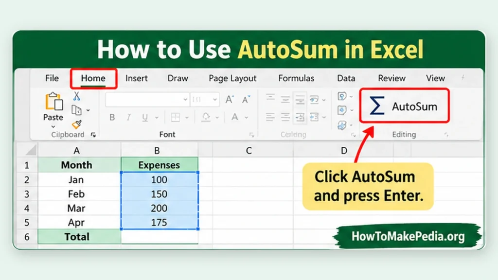
AutoSum automatically inserts a SUM formula. It is especially useful when you have a column or row of numbers and don’t want to type the references yourself.
Follow these steps:
- Open your worksheet.
- Select the empty cell below your numbers.
- Click the Home tab.
- Select AutoSum (∑).
- Check the highlighted range.
- Press Enter to confirm.
You can also find AutoSum on the Formulas tab.
For example, if cells C2 through C8 contain expenses, clicking AutoSum in C9 may create:
=SUM(C2:C8)
Can AutoSum Add Multiple Columns?
Yes. If several adjacent columns contain numeric data, you can select the empty total cells beneath them and click AutoSum. Excel can create a separate SUM formula for each column.
Important: AutoSum might stop selecting cells when it encounters a blank row or column. Always check the highlighted range before confirming the formula.
Method 3: Excel SUM Keyboard Shortcut
If you frequently work with numerical data, the AutoSum keyboard shortcut can save you time.
Windows Shortcut: Alt + =
- Select the empty cell where the total should appear.
- Press Alt + =.
- Review the suggested range.
- Press Enter.
Excel inserts a SUM formula without requiring you to type the function name.
Mac Shortcut
In supported desktop versions of Excel for Mac, Shift + Command + T inserts AutoSum.
Shortcuts may behave differently in browser-based Excel, so the AutoSum button is a reliable alternative when a keyboard combination doesn’t work.
Method 4: Sum Numbers Using the Excel Status Bar
Sometimes you only need to check a total rather than save it in your worksheet.
The Excel Status Bar can do this quickly.
- Select the cells containing the numbers.
- Look at the bottom of the Excel window.
- Find the value labeled Sum.
- Read the calculated result.
For example, selecting cells containing 20, 40, and 60 displays a sum of 120.
On Excel for Windows desktop, if Sum is missing, right-click the Status Bar and enable the Sum option.
Unlike a SUM formula, the Status Bar result is temporary. It does not place a calculated value in a worksheet cell.
Method 5: Sum Data Using an Excel Table Total Row
If your spreadsheet contains a growing list of sales or expenses, an Excel Table can make total calculations easier to manage.
Here’s how:
- Select your data, including any column headers.
- Go to Insert > Table, or press Ctrl + T in Excel for Windows.
- Confirm the correct data range and header setting.
- Click inside the newly created table.
- Open Table Design and enable Total Row.
- Use the drop-down in the appropriate total cell to select Sum.
Excel Tables can expand as you add records, keeping your calculations organized.
A Table Total Row commonly uses a SUBTOTAL formula rather than an ordinary SUM formula. This matters when you filter records because the displayed total can adjust to the visible rows.
Before adding up a sales report, check whether repeated records are genuine transactions or accidental duplicates. If necessary, follow our guide on how to remove duplicates in Excel to clean up your data without accidentally deleting valid entries.
How to Sum a Column in Excel
To add a vertical list of numbers, use the SUM function with a column range.
For example:
=SUM(B2:B20)
This adds every numeric value from B2 through B20.
Place the formula in B21 or another cell outside the selected range.
You can also use:
=SUM(B:B)
This references the entire B column. However, don’t place that formula anywhere in column B because it would include its own cell and create a circular reference.
For everyday worksheets, a specific range is usually easier to review.
How to Sum a Row in Excel

To add values arranged horizontally, use a row range.
Suppose cells B2 through G2 contain six expense amounts.
Enter:
=SUM(B2:G2)
Excel adds all six values.
You can place the formula in H2, directly to the right of the final expense.
AutoSum also works horizontally when the result cell is beside the numbers.
If your expense categories have lengthy names, you can improve the worksheet’s appearance using our guide on how to wrap text in Excel. Wrapped headings make budget tables easier to read without changing calculations.
How to Sum Multiple Cells in Excel
Sometimes the cells you want to add are separated by other data.
You don’t need to move them next to each other.
Use:
=SUM(B2,D2,F2)
This adds only B2, D2, and F2.
For example, if those cells contain 100, 75, and 25, the result is 200.
The commas separate individual cell references. Depending on your regional Excel settings, you may need to use semicolons instead.
How to Sum Multiple Columns or Ranges
You can combine several ranges in one SUM formula.
For example:
=SUM(B2:B10,D2:D10)
This adds the values in both ranges.
Imagine column B contains online sales while column D contains in-store sales. This formula calculates their combined total without including columns C or E.
Avoid accidentally selecting overlapping ranges, such as B2:B10 and B5:B12, because some values would be counted twice.
How to Calculate a Running Total in Excel
A running total shows how the cumulative amount changes after each new entry.
Suppose you have daily expenses in column B and want cumulative spending in column C.
| Cell | Expense | Running Total |
|---|---|---|
| Row 2 | $100 | $100 |
| Row 3 | $75 | $175 |
| Row 4 | $125 | $300 |
In cell C2, enter:
=SUM($B$2:B2)
Then drag the fill handle down to copy the formula.
Excel adjusts the ending reference while keeping the starting reference fixed:
- C2:
=SUM($B$2:B2)→ 100 - C3:
=SUM($B$2:B3)→ 175 - C4:
=SUM($B$2:B4)→ 300
The dollar signs in $B$2 lock the starting cell. Without them, both ends of the range could move when you copy the formula downward.
Running totals are useful for monitoring cumulative sales, monthly spending, savings, and inventory movements.
How to Sum Only Visible or Filtered Rows

A regular SUM formula includes numerical values even when some rows are hidden.
For example:
=SUM(B2:B20)
This calculates the total for the entire selected range, including rows hidden manually or by filtering.
If you want to add only visible values in a vertical range, use:
=SUBTOTAL(109,B2:B20)
Here, 109 tells Excel to perform a SUM calculation while excluding filtered-out and manually hidden rows.
SUM vs. SUBTOTAL Example
Imagine this sales report:
| Region | Sales |
|---|---|
| East | $100 |
| West | $200 |
| East | $150 |
The regular SUM result is $450.
If you filter the worksheet to show only East, SUBTOTAL(109,...) returns $250, while an ordinary SUM of the original range still returns $450.
You can also use SUBTOTAL(9,B2:B20). This excludes filtered-out rows but includes manually hidden rows.
If you’re working with large reports, read our tutorial on how to hide rows in Excel to understand how row visibility works.
SUM vs. SUMIF vs. SUMIFS vs. SUBTOTAL
Excel has several functions for adding data. Choosing the correct one depends on whether you need conditions or want to exclude hidden rows.
| Function | Purpose | Example |
|---|---|---|
| SUM | Adds numbers in a range | =SUM(B2:B10) |
| SUMIF | Adds numbers matching one condition | =SUMIF(A2:A10,"East",B2:B10) |
| SUMIFS | Adds numbers matching multiple conditions | =SUMIFS(C2:C10,A2:A10,"East",B2:B10,"Paid") |
| SUBTOTAL | Adds data while accounting for row visibility | =SUBTOTAL(109,B2:B10) |
In the SUMIF example, column A contains regions and column B contains sales.
In the SUMIFS example, column A contains regions, column B contains payment statuses, and column C contains sales amounts. The formula adds sales that are both East and Paid.
Use SUM for ordinary addition, SUMIF or SUMIFS for conditional totals, and SUBTOTAL when row visibility affects the answer.
How to Sum in Excel on Mac and Excel for the Web
The standard formula works in supported desktop and web versions of Microsoft Excel:
=SUM(A2:A10)
On a Mac, type the formula and press Return. You can also select AutoSum from the Ribbon or use its supported keyboard shortcut.
In Excel for the web, enter a SUM formula or use the AutoSum button. Browser shortcuts can vary because some key combinations are handled by the browser.
Regional settings may also change formula separators. If Excel rejects commas between arguments, check whether your configuration expects semicolons.
Why Is My SUM Formula Not Working in Excel?
Most SUM problems come from incorrect references, text-formatted data, or workbook calculation settings.
1. Numbers Are Stored as Text
Imported values may look like numbers but actually be stored as text.
Excel generally ignores these values when they appear in a referenced SUM range.
Fix: Check for an error indicator and use Convert to Number when available. You can also use an appropriate data conversion method, such as Text to Columns, after checking the source values.
Changing only the display format does not always convert existing text into real numbers.
2. SUM Returns Zero
If a formula returns zero unexpectedly, the referenced cells might contain numeric-looking text rather than actual numbers.
Fix: Confirm that the selected range contains numeric values and correct any text-number issues.
3. Excel Displays the Formula Instead of the Result
For example, you might see =SUM(B2:B6) rather than 600.
Fix: Make sure the cell is not formatted as Text, change it to General if necessary, and re-enter the formula. Also check whether Formulas > Show Formulas is enabled.
4. AutoSum Selects the Wrong Range
Blank rows or nearby numbers can cause Excel to suggest an incomplete or unintended range.
Fix: Edit the references inside the SUM formula before pressing Enter.
5. The Formula Does Not Recalculate
Your workbook may be using manual calculation.
Fix: In Excel desktop, go to Formulas > Calculation Options > Automatic. You can also use Calculate Now to refresh formulas.
6. A Circular Reference Appears
This happens when a formula includes its own result cell.
For example, putting =SUM(B2:B10) in B10 creates a circular reference.
Fix: Move the formula to B11 or change the range so it excludes the result cell.
7. Excel Shows a #VALUE! Error
Using =B2+B3 may produce an error when one referenced cell contains incompatible text.
By comparison, =SUM(B2:B3) generally ignores text stored in referenced cells.
Fix: Check referenced values and correct invalid inputs. Remember that errors already present within a referenced range can also affect SUM results.
8. Excel Shows a #REF! Error
A #REF! error indicates an invalid cell reference, possibly caused by deleting cells or changing the worksheet structure.
Fix: Inspect the formula and replace broken references with valid cells or ranges.
Hiding rows does not automatically remove their values from a regular SUM calculation.
Fix: Use =SUBTOTAL(109,B2:B20) when you need a visible-row total.
Also, marking a completed or canceled expense with strikethrough does not remove its numeric value from SUM. If you use visual formatting in an expense tracker, our how to strikethrough in Excel guide explains the formatting steps. Use a separate status column or an appropriate conditional formula when you need to exclude canceled expenses from totals.
How to Sum Across Different Worksheets
You can calculate a combined total from several worksheets in the same Excel workbook.
For example:
=SUM(January!B2,February!B2,March!B2)
This adds cell B2 from three sheets named January, February, and March.
The exclamation mark separates the worksheet name from its cell reference.
If your worksheets share the same structure, you can also use a 3-D reference such as:
=SUM(January:March!B2)
This includes B2 from every sheet positioned between January and March, including the endpoints.
Use this approach only when the intervening sheets contain the values you intend to add.
Common Mistakes When Using SUM
Before finalizing a spreadsheet, check for these mistakes:
- Leaving out the equal sign before a formula.
- Using commas instead of a colon for a continuous range.
- Selecting incomplete ranges.
- Including the result cell in its own formula.
- Counting overlapping ranges twice.
- Treating imported text as numbers.
- Assuming filtered or hidden values are excluded.
- Using SUM when the task actually requires SUMIF or SUBTOTAL.
- Selecting the wrong worksheet in a cross-sheet formula.
- Expecting a temporary Status Bar total to be saved automatically.
Reviewing the cell references is often the quickest way to identify a wrong total.
Frequently Asked Questions
How do I sum numbers in Excel?
Select an empty cell, type =SUM(A2:A10), and press Enter to add the numeric values in that range.
What is the SUM formula in Excel?
The SUM function uses the syntax =SUM(number1,[number2],...) to add numbers, references, and ranges.
How do I sum an entire column?
Use a range such as =SUM(B2:B100). You can also reference an entire column with =SUM(B:B) if the formula is outside column B.
How do I sum a row?
Use =SUM(B2:G2) to add values across a horizontal range.
What is the shortcut for SUM in Excel?
Press Alt + = in Excel for Windows. A supported shortcut in Excel for Mac is Shift + Command + T.
How do I use AutoSum?
Select the empty cell beside or below your numbers, click Home > AutoSum, verify the selected range, and press Enter.
How do I add separate cells?
Use =SUM(B2,D2,F2) to add nonadjacent cells.
Can I sum multiple ranges?
Yes. Use a formula such as =SUM(B2:B10,D2:D10).
How do I calculate a running total?
In C2, enter =SUM($B$2:B2) and copy the formula downward. The starting reference remains fixed while the ending reference expands.
How do I sum only visible rows?
Use =SUBTOTAL(109,B2:B20) for a vertical range to exclude filtered-out and manually hidden rows.
Why does SUM return zero?
The cells may contain numeric-looking text, the formula may reference the wrong range, or the numerical values may genuinely total zero.
Why isn’t Excel updating my total?
Check whether workbook calculation is set to Manual. Switching to Automatic usually restores recalculation when referenced values change.
What is the difference between SUM and SUMIF?
SUM adds numbers without applying criteria. SUMIF adds only the values that match one specified condition.
Yes. Ordinary SUM formulas include numbers in hidden and filtered-out rows.
Can I use SUM in Excel Online?
Yes. Excel for the web supports the SUM function and AutoSum.
Conclusion
The easiest way to add numbers in Excel is to use the SUM function. It works for individual cells, complete rows, columns, and multiple ranges. AutoSum and the Alt + = Windows shortcut provide faster alternatives when you need a quick total.
For cumulative calculations, use a running total formula with a fixed starting reference. If your worksheet contains filtered or hidden data, use SUBTOTAL when you want the result to reflect visible rows.

1 Comment
Pingback: How to Calculate Average of Average in Excel (2 Methods)